COVID-19 NYC MTA Mobility Trends 2019 vs 2020
An Exploration of the Impact of the COVID-19 Pandemic on Mobility as Measured by MTA Ridership
Contributors: Michelle Lee, Julián Ponce, Adarsh Ramakrishnan, Allison Stewart, Aishwarya Anuraj (MPH candidates at Columbia University)
Project Motivation
The central artery of New York City, the public transportation system is central to the city’s cultural and economic well-being. Among its usual million daily users such as hip hop dancers, Wall Street executives, and the famous pizzarat, the subway proves to be more than a means of transport; it is a way of life.
Unfortunately, the COVID-19 pandemic and the “New York State on PAUSE” executive order, issued on March 14, 2020 aimed to slow the spread of the virus, brought tremendous shock to the normal bustle of New York City. Closed museums, theaters, restaurants, and suspended commutes have created ghost town-like scenes and some people to proclaim that New York City is “over” as we know it.
This project moves forward with the aim of understanding the influence of the COVID-19 pandemic on mobility trends in NYC as measured by MTA ridership on subway trains and buses from March to November 2019 and 2020.
Understanding this important issue could provide insight to policymakers, transit authorities, and health departments as they make decisions related to transmission of COVID-19 and modifications to public transportation systems in light of stay-at-home orders.
Research Questions
- How has the COVID-19 pandemic influenced trends in subway and bus ridership in NYC from March to November 2020?
- Does average MTA subway ridership from March to November 2019 differ from MTA subway ridership from March to November 2020?
- Does subway ridership differ from bus ridership during the COVID-19 pandemic (March to November 2020)?
Mobility Analysis
We used a publicly available dataset on day-by-day ridership numbers from the MTA. The dataset contains information on total estimated ridership and percentage change from 2019 by day, beginning March 1, 2020. Estimates of ridership by subway, bus (local, limited, SBS, and Express), Long Island Rail Road, Metro-North Railroad, Access-A-Ride, and Bridges and Tunnels are all available, however, we decided to restrict our analysis to subway and bus ridership.
knitr::opts_chunk$set(echo = TRUE)
library(tidyverse)
library(patchwork)
library(readr)
library(broom)
library(dbplyr)
library(viridis)
library(reshape2)
library(plotly)
library(lubridate)
knitr::opts_chunk$set(
    echo = TRUE,
    warning = FALSE,
    fig.width = 8,
  fig.height = 6,
  out.width = "90%"
)
options(
  ggplot2.continuous.colour = "viridis",
  ggplot2.continuous.fill = "viridis"
)
scale_colour_discrete = scale_colour_viridis_d
scale_fill_discrete = scale_fill_viridis_d
theme_set(theme_minimal() + theme(legend.position = "bottom"))

mta_data = read_csv (file = "./data/MTA_recent_ridership_data_20201123_0.csv",
                     col_types = cols(
                       date = col_date(format = "%mm/%dd/%yy"),
                       `Subways: % Change From 2019 Equivalent Day` = col_number(),
                       `Buses: % Change From 2019 Equivalent Day` = col_number(),
                       `Bridges and Tunnels: % Change From 2019 Equivalent Day` = col_number()
                       ) #only changed the formats of important variables
) %>%
  janitor::clean_names()
skimr::skim(mta_data)
mta_data =
  mta_data %>%
  subset(select = -c(lirr_total_estimated_ridership, lirr_percent_change_from_2019_monthly_weekday_saturday_sunday_average, metro_north_total_estimated_ridership, metro_north_percent_change_from_2019_monthly_weekday_saturday_sunday_average, access_a_ride_total_scheduled_trips, access_a_ride_percent_change_from_2019_monthly_weekday_saturday_sunday_average, bridges_and_tunnels_total_traffic, bridges_and_tunnels_percent_change_from_2019_equivalent_day))
#exclude data for lirr, metronorth, access-a-ride, bridges & tunnel
#calculate 2019 ridership data
mta_data = mta_data %>%
  mutate(
    'subway_2019' = subways_total_estimated_ridership/(1+(subways_percent_change_from_2019_equivalent_day/100)),
    'bus_2019'=
      buses_total_estimated_ridership/(1+(buses_percent_change_from_2019_equivalent_day/100))
    ) %>%
  rename(
    "subway_2020" = subways_total_estimated_ridership,
    "subway_pct_change" = subways_percent_change_from_2019_equivalent_day,
    "bus_2020" = buses_total_estimated_ridership,
    "bus_pct_change" = buses_percent_change_from_2019_equivalent_day
    )
#change date to date format and order by date
plot_mta =
mta_data %>%
mutate(
date= as.Date(date,format = "%m/%d")) %>%
arrange(date)
#create a text_label label
text_label =
plot_mta %>%
mutate(text_label = str_c("percent change from 2019 to 2020: ", subway_pct_change)) %>%
select(date, text_label)
#graph for subway
#pivoting
plot_subway =
plot_mta %>%
select(subway_2020, subway_2019, date) %>%
melt(., id.vars = "date") %>%
#merge based on month
merge(text_label, by = "date") %>%
#plotting
plot_ly(
x = ~date, y = ~value, type = "scatter", mode = "markers",
color = ~variable, text = ~text_label) %>%
layout (
title = "Figure 2. Subway Ridership Trends 2019 - 2020",
xaxis = list(title ="Month/Day", tickformat = "%m/%d"), #drop year
yaxis = list(title="Ridership")) %>%
add_lines(x =as.Date("2020-03-01"), line = list(dash="dot", color = 'red', width=0.5, opacity = 0.5),name = 'First case on 3/1') %>%
add_lines(x =as.Date("2020-04-07"), line = list(dash="dot", color = 'red', width=0.5, alpha = 0.5),name = '100K cases in NYC on 04/07') %>%
add_lines(x =as.Date("2020-05-26"), line = list(dash="dot", color = 'red', width=0.5, alpha = 0.5),name = '200K cases in NYC on 05/26')
#graph for bus
#pivoting
plot_bus =
plot_mta %>%
select(bus_2020,bus_2019,date) %>%
melt(., id.vars = "date") %>%
#merge based on month
merge(text_label, by = "date") %>%
#plotting
plot_ly(
x = ~date, y = ~value, type = "scatter", mode = "markers",
color = ~variable, text = ~text_label) %>%
layout (
title = "Figure 1. Bus Ridership Trends 2019 - 2020",
xaxis = list(title ="Month/Day", tickformat = "%m/%d"),
yaxis = list(title="Ridership")) %>%
add_lines(x =as.Date("2020-03-01"), line = list(dash="dot", color = 'red', width=0.5, opacity = 0.5),name = 'First case on 3/1') %>%
add_lines(x =as.Date("2020-04-07"), line = list(dash="dot", color = 'red', width=0.5, alpha = 0.5),name = '100K cases in NYC on 04/07') %>%
add_lines(x =as.Date("2020-05-26"), line = list(dash="dot", color = 'red', width=0.5, alpha = 0.5),name = '200K cases in NYC on 05/26')
#ggplot for subway
plot_subway_2 =
plot_mta %>%
select(subway_2020, subway_2019, date) %>%
melt(., id.vars = "date") %>%
ggplot(aes(x=date, y=value, color=variable)) +
geom_point(alpha=0.5) +
geom_smooth(se = FALSE) +
xlab("Month/Day") +
ylab("Ridership") +
ggtitle("Subway Ridership Trends 2019 - 2020") +
geom_vline(xintercept=as.Date("2020-03-01"), linetype="dotted", color = 'red')+
geom_vline(xintercept=as.Date("2020-04-07"), linetype="dotted", color = 'red')+
geom_vline(xintercept=as.Date("2020-05-26"), linetype="dotted", color = 'red')+
geom_text(x=as.Date("2020-03-01"), y=6100000, label ="First case", angle=90, vjust = 1.2, size=3,color='black') +
geom_text(x=as.Date("2020-04-07"), y=6100000, label ='100K cases', angle=90, vjust = 1.2, size=3,color='black')+
geom_text(x=as.Date("2020-05-26"), y=6100000, label ='200K cases', angle=90, vjust = 1.2, size=3,color='black')
#ggplot for bus
plot_bus_2 =
plot_mta %>%
select(bus_2020, bus_2019,date) %>%
melt(., id.vars = "date") %>%
ggplot(aes(x=date, y=value, color=variable)) +
geom_point(alpha=0.5) +
geom_smooth(se = FALSE) +
xlab("Month/Day") +
ylab("Ridership") +
ggtitle("Bus Ridership Trends 2019 - 2020") +
geom_vline(xintercept=as.Date("2020-03-01"), linetype="dotted", color = 'red')+
geom_vline(xintercept=as.Date("2020-04-07"), linetype="dotted", color = 'red')+
geom_vline(xintercept=as.Date("2020-05-26"), linetype="dotted", color = 'red')+
geom_text(x=as.Date("2020-03-01"), y=2400000, label ="First case", angle=90, vjust = 1.2, size=3,color='black') +
geom_text(x=as.Date("2020-04-07"), y=2400000, label ='100K cases', angle=90, vjust = 1.2, size=3,color='black')+
geom_text(x=as.Date("2020-05-26"), y=2400000, label ='200K cases', angle=90, vjust = 1.2, size=3,color='black')#see the two graphs together:
plot_busplot_subway(plot_bus_2+plot_subway_2 + plot_annotation(
title = 'Figure 3. Bus and Subway Ridership Trends 2019-2020', theme = theme(plot.title = element_text(size = 20)
)))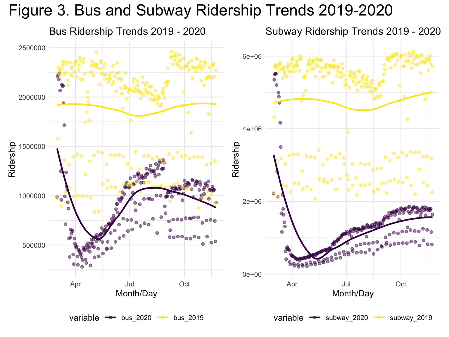
Highlights:
Overall reduction in bus and subway ridership in 2020 compared to 2019
Substantial drop in bus and subway ridership from March to April 2020
Fewer people chose to use the subway as compared to buses after April, 2020
In Figure 1., which shows trends in bus ridership, there appears to be a continuous drop in ridership between the first COVID-19 case on March 1, 2020 and April 1, 2020. This trend is followed by an increase in ridership in April through July 2020 and then subsequently a broadening of the range of values around August 2020, with some reductions in values and others remaining generally constant. From the 2019 estimates, we also notice many outlying lower values, produced by decreased bus ridership on Thursdays and Fridays. This is likely a result of fewer commuters on those days.
In Figure 2., which shows trends in subway ridership, there appears to be similarities to the bus ridership trends from Figure 1. However, there are fewer overlapping values when comparing the years 2019 and 2020. The increase in subway ridership, beginning around April 2020 is also less extreme than the increase in bus ridership and there is a more narrow range of values in the 2020 subway ridership as compared to bus ridership. Finally, the 2020 subway ridership does not appear to be decreasing in recent months as with bus ridership. These trends suggest that as people began to use public transportation again during the pandemic, fewer people chose to use the subway as compared to buses.
In Figure 3. we observe that from mid-March onward there are overall reduced ridership trends in 2020 as compared to 2019 for both forms of transit.
Statistical Analysis
We conducted a two-sample t-test to explore the difference in average subway ridership between 2019 and 2020.
#separate by month and day
mta_data =
  mta_data %>%
  arrange(date) %>%
  separate(date, into = c("month", "day", "year"))%>%
  mutate(month = as.numeric(month),
         day = as.numeric(day)) %>%
  select(-c(year)) #drop year column
mta_subway_ridership =
  mta_data %>%
  group_by(month)%>%
  summarize(
    avg_subway_2019 = mean(subway_2019),
    avg_subway_2020 = mean(subway_2020)
  )
mta_subway_ridership%>%knitr::kable()
mta_2019_sample =
  mta_data%>%
  select(month, subway_2019) %>%
  nest(subway_2019)%>%
  mutate("subway_2019_sample" = data)%>%
  select(-data)
mta_2020_sample =
  mta_data%>%
  select(month, subway_2020)%>%
  nest(subway_2020)%>%
  mutate("subway_2020_sample" = data)%>%
  select(-data)
mta_samples =
  bind_cols(mta_2019_sample, mta_2020_sample)%>%
  select(-month...3)%>%
  rename(month = month...1)

mta_t_test =
  mta_samples%>%
  mutate(t_test = map2(.x = subway_2019_sample, .y = subway_2020_sample, ~t.test(.x , .y) ),
         t_test_results = map(t_test, broom::tidy))%>%
  select(month, t_test_results)%>%
  unnest(t_test_results)%>%
  select(month,p.value)%>%
  mutate(difference = case_when(
    p.value >= 0.05 ~ "insignificant",
    p.value < 0.05 ~ "significant"),
    p.value = ifelse(
    p.value< 0.001,"<0.001",round(p.value, digits = 4))) %>%
  arrange(month)
knitr::kable(mta_t_test, digits = 3)
Table 1. T-test Results by Month
Merged t-test results with the average ridership for each month.
mta_year_ttest =
  bind_cols(mta_subway_ridership, mta_t_test)%>%
  select(-month...4)%>%
  rename(month = month...1)
knitr::kable(mta_year_ttest)| month | avg_subway_2019 | avg_subway_2020 | p.value | difference |
|---|---|---|---|---|
| 3 | 4746353 | 2381477.6 | <0.001 | significant |
| 4 | 4873551 | 391671.7 | <0.001 | significant |
| 5 | 4682924 | 493526.1 | <0.001 | significant |
| 6 | 4883863 | 798982.6 | <0.001 | significant |
| 7 | 4516652 | 1050498.6 | <0.001 | significant |
| 8 | 4343573 | 1137601.2 | <0.001 | significant |
| 9 | 4886223 | 1428918.6 | <0.001 | significant |
| 10 | 4964620 | 1549459.3 | <0.001 | significant |
| 11 | 4879758 | 1522150.0 | <0.001 | significant |
The following plot was created using the final data frame to depict average ridership for each month comparing 2019 and 2020. The labels that appear at each data point as you hover over them provide additional information about the significance or lack of significance in ridership difference.
Figure 4. Monthly Average Ridership of Subway 2019 vs 2020
#create a text_label label
text_label =
  mta_year_ttest %>%
  mutate(text_label = str_c("p-value: ",p.value, "\nDifference: ", difference)) %>%
  select(month, text_label)
#pivoting
plot_ttest =
  mta_subway_ridership %>%
  rename(
    "2020"=avg_subway_2020,
    "2019"=avg_subway_2019
  ) %>%
  melt(., id.vars = "month") %>%
#merge based on month
  merge(text_label, by = "month")
#plotting
plot_ttest %>%
plot_ly(
    x = ~month, y = ~value, type = "scatter", mode = "lines+markers",
    color = ~variable, text = ~text_label) %>%
  layout (
    title = "Monthly Average Ridership of Subway 2019 vs 2020",
    xaxis = list(title ="Months",range=c(3,11)),
    yaxis = list(title="Average Ridership"))
The results indicate that there is a statistically significant difference (p <.001) in subway ridership trends across all months(March-November)in 2019 and 2020.
Regression
Next, we proposed a regression model for subway ridership in 2020.
subway_ridership = lm(subway_2020 ~ month, data = mta_data)
subway_ridership %>%
  broom::tidy()
## # A tibble: 2 × 5
## term estimate std.error statistic p.value
## <chr> <dbl> <dbl> <dbl> <dbl>
## 1 (Intercept) 965080. 160401. 6.02 0.00000000587
## 2 month 32473. 21860. 1.49 0.139#to tidy the output and get only the intercept, slope and p-values
subway_ridership %>%
broom::tidy() %>%
select(term, estimate, p.value) %>%
knitr::kable(digits = 3)| term | estimate | p.value |
|---|---|---|
| (Intercept) | 965079.87 | 0.000 |
| month | 32472.74 | 0.139 |
#to plot for regression line
  ggplot(mta_data, aes(month, subway_2020)) +
  geom_point() +
  stat_smooth(method = lm)+
   xlab("Month in 2020") +
  ylab("Subway Ridership") +
  ggtitle(" Figure 5. Subway Ridership 2020 Regression")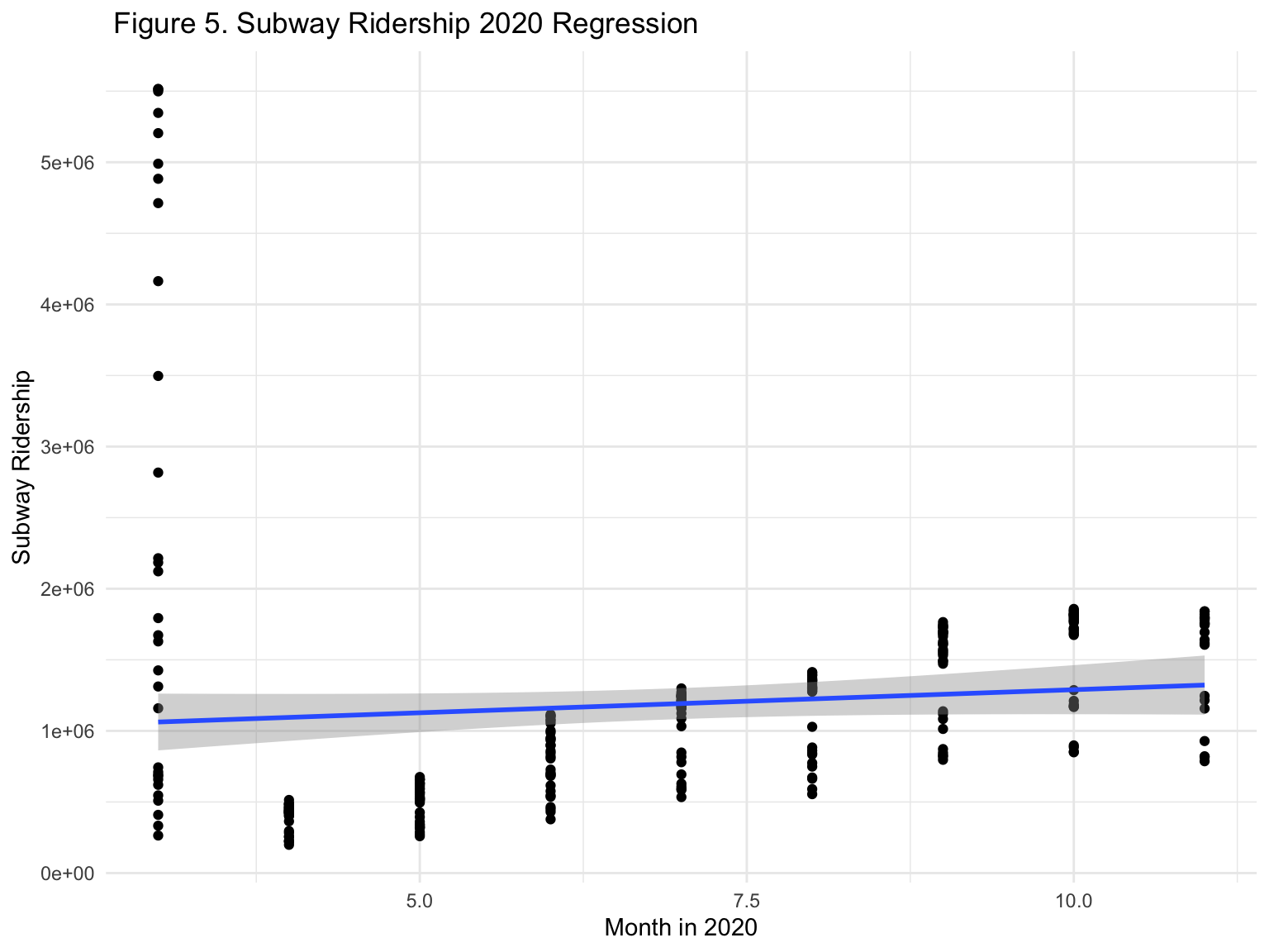
Then, we built a plot of model residuals against fitted values for subway ridership and bus in 2020.
mta_data %>%
  modelr::add_predictions(subway_ridership) %>%
  modelr::add_residuals(subway_ridership) %>%
  ggplot(aes(x = pred, y = resid)) + geom_point() +
  labs(x = "Predicted value",
       y = "Residual") +
    ggtitle("Figure 6. Residual vs. Predicted value of Subway 2020 Ridership Regression Model")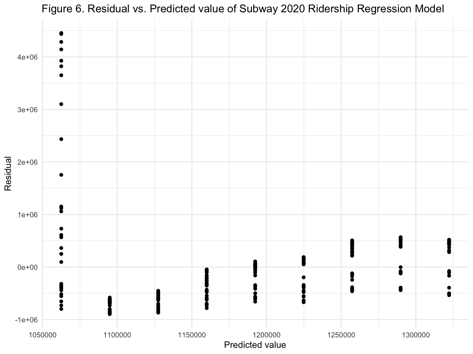
bus_ridership = lm(bus_2020 ~ month, data = mta_data)
bus_ridership %>%
  broom::tidy()
## # A tibble: 2 × 5
## term estimate std.error statistic p.value
## <chr> <dbl> <dbl> <dbl> <dbl>
## 1 (Intercept) 717060. 64077. 11.2 4.46e-24
## 2 month 26325. 8733. 3.01 2.82e- 3#Now we need to tidy the output and get only the intercept, slope and p-values
bus_ridership %>%
broom::tidy() %>%
select(term, estimate, p.value) %>%
knitr::kable(digits = 3)| term | estimate | p.value |
|---|---|---|
| (Intercept) | 717060.27 | 0.000 |
| month | 26324.69 | 0.003 |
#to plot for regression line
ggplot(mta_data, aes(month, bus_2020)) +
  geom_point() +
  stat_smooth(method = lm)+
   xlab("Month in 2020") +
  ylab("Bus Ridership") +
  ggtitle(" Figure 7. Bus Ridership 2020 Regression")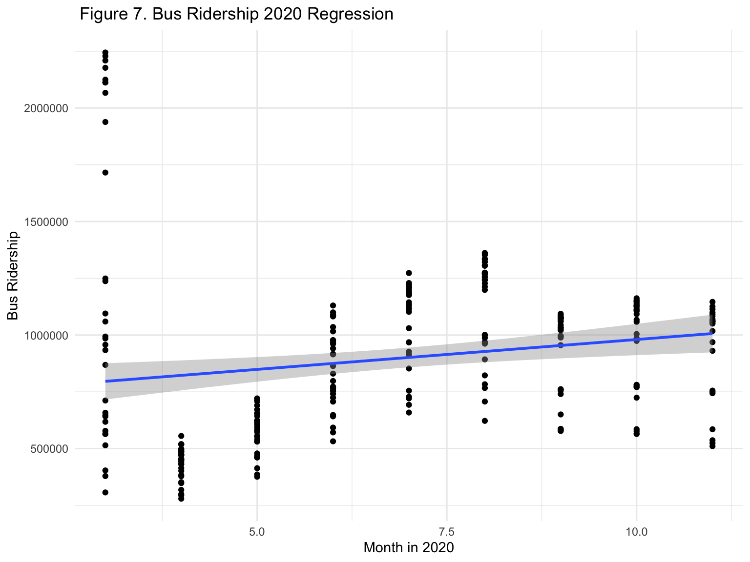
Next, we will built a plot of model residuals against fitted values for bus ridership in 2020.
mta_data %>%
  modelr::add_predictions(bus_ridership) %>%
  modelr::add_residuals(bus_ridership) %>%
  ggplot(aes(x = pred, y = resid)) + geom_point() +
  labs(x = "Predicted value",
       y = "Residual")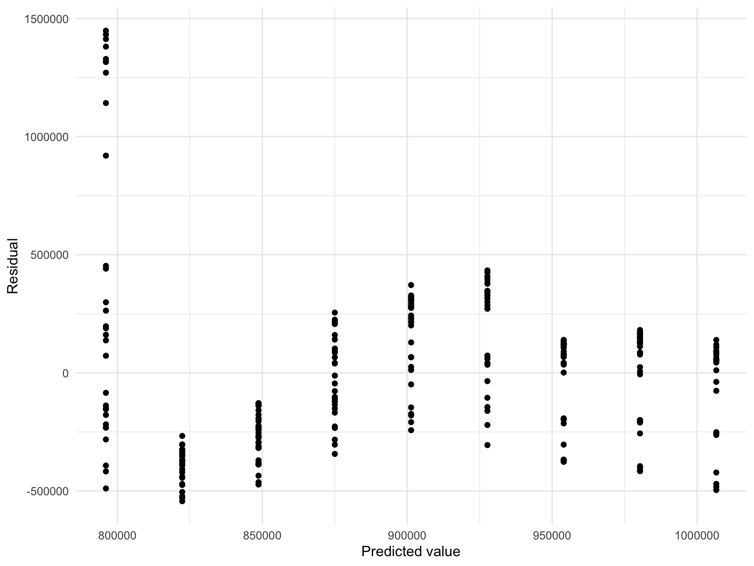
ggtitle("Residual vs. Predicted value of Subway 2020 Ridership Regression Model")## $title
## [1] "Residual vs. Predicted value of Subway 2020 Ridership Regression Model"
##
## attr(,"class")
## [1] "labels"Results
- Subway
- For each additional change in month, we expect subway ridership to increase by 32,473 units, on average.
- Bus
- For each additional change in month, we expect bus ridership to increase by 26,325 units, on average.
Discussion
Analysis using t test support our hypothesis that the average MTA subway ridership in 2020 was significantly different from that of 2019. We further observe in the regression analysis that as months progressed there were increases in both subway and bus ridership.
From mid-March onward, there are overall reduced ridership trends in 2020 as compared to 2019 for both forms of transit.There is a steep decline in ridership starting late March/ Early April. This could be due to (1) the statewide PAUSE order where people who were not essential workers did not use MTA to commute to work,(2) closing of schools, in which millions of students use MTA to go to school, and (3) decline in tourism. We can observe an increase in ridership for both subway and bus, starting early June. This could be due to (1) people are going back to school and work, and (2) people feel comfortable using public transportation as the rates of infection in New York City slowed down, compared to March - late May, where we reached 200,000 cumulative cases for COVID-19 within 50 days.
The implications of our findings are valuable in understanding the impact of COVID-19 on usage of public transportation in NYC. Our findings could provide insight to transit authorities in regards to changes in schedules in light of recent budget cuts. Health departments and contact traces could benefit from using these findings about population movements and density to better understand future outbreaks of COVID-19. Most importantly, state officials can understand how measures such as stay at home orders can influence overall transit density and consumer spending.
Further studies should examine additional modes of transportation such as personal vehicles, air traffic, and bike usage. Analysis broken down by borough could provide further details on mobility trends among neighborhoods of different socio-economic status.